SVM (Support Vector Machines) Modelling

• SVM is a linear regression model
• Helps in dealing with large volume & high dimension
• Not suitable for imbalanced data (why?) 
• SVM on imbalanced data often produces models that are biased towards majority data and hence poor performance on minority data.
• Tips on choosing the right type of kernel for SVM
• Ultimately boils down to trial and error
• But not completely random, lot of this is informed by experience
• You would get a sense what the classification boundary would look like when doing the EDA
• If you find that data plot is completely intermingled, then non-linearity is needed.
• If the data points are reasonably separable by a linear hyperplane, more or less, then linearity should do. 
• If there is a reasonable curvy line you could draw as a separator, then a polynomial kernel should work.
• If the data is hopelessly intermingled, you would need a complex kernel. A most common choice in this case is an RBF Kernel.
• 
  

SVM Notations

• 2-D hyperplane (essentially a line when it comes to 2-D) equation
  W0 + W1X1 + W2X2 = 0
• n-D equation
• 
  

General ML Notes

Resources

Model Building

1. Dummy Variables
2. Why it's necessary to create dummy variables 
3. When to Normalise date and when to standardise? 
4. Scaling techniques

Model Comparison (R-squared normalisation techniques)

1. AIC (Akaike Information Criterion)
2. BIC (Bayesian Information Criterion)
3. Mallow's Cp

Feature Selection

1. univariate methods
2. linear models and regularization
3. random forests
4. stability selection, rfe and the above compared

Exploratory Data Analysis

Sources of Public Data

• GitHub: Awesome Public Datasets 
• Open Government Data (OGD) Platform India
• GitHub: DataMeet

Hypothesis Testing

Notes

• Null Hypothesis: The one that pertains to the status quo, typically the original claim (if the original claim causes the Null Hypothesis to not have an = sign in the statement, then it is flipped). So, typically µ >= / <= / = a value.

• Alternate Hypothesis: Complements the Null Hypothesis. If proven, you reject the Null Hypothesis.
• p-Value, in layman's terms, can be defined as the Probablity that the Null hypothesis is correct
• 
  

Inferential Stats

Notes

• Normal Distribution
• Most naturally occurring phenomena follow a normal distribution i.e. a bell curve
• The bell curve has many interesting features
• The mean & mode coincide
• The 1-2-3 rule
• The probability of any value lying within 1 standard deviation (sigma σ) from the mean (mu µ) is 68% (i.e µ+1 σ or µ-1 σs).
• The probability of any value lying within 2 standard deviations (sigma) from the mean (mu) is 95% (i.e µ+2 σ or µ-2 σ).
• The probability of any value lying within 3 standard deviations (sigma) from the mean (mu) is 99.7% (i.e µ+3 σ or µ-3 σ).
• As a convention, a random variable's (X) value is specified in terms of its distance from the mean µ in units of std deviation σ i.e., (X-µ)/σ units - this is called Z, the standardised normal variable.
  e.g if, say, µ is 35 and σ is 5, X value of 43.5  would be (43.5 - 35)/5 units = 1.7σ away from mean. Hence Z score is 1.7
• (Ugly) Alternative to Z Score table
   (Z)=1√2π∫Z−∞e−t22dt
• or in Excel, NORM.S.DIST(z, TRUE/FALSE) where
  TRUE means find the cumulative probability, FALSE means find the probability density.

• Sampling
• When dealing with large populations, it is more feasible to quantify the characteristics of the population by using "samples" of the population.
• Working with the samples, we can approximate/extrapolate the characteristics of the original, full population
• Sampling distributions play an important part in understanding the "margin of error" and our confidence to closeness to the population when inferring chracteristics.
• A sampling distribution starts to approach/resemble a normal distribution at a sampling size (n) of 30.

•  The Central Limit Theorem (CLT)
• For any kind of data (regardless of how it is distributed viz. normal, skewed, uniform etc.), the following properties hold true, provided a high number of samples has been taken :
1. Sampling distribution's mean (µ⎺X) = Population mean (µ)
2. Sampling distribution's standard deviation (Standard error) = σ / √n
3. For n > 30, the sampling distribution becomes a normal distribution.

Resource Links

• Statistical Inference for Data Science
• Seeing Theory
• Z-Score table
• Exponential Distribution
• Gamma Distribution
• Chi-Squared Distribution
• http://onlinestatbook.com/stat_sim/sampling_dist/index.html
• Math for grownups - Exit polling: A statistics refresher
• University of Warwick - Exit polling explained

Resources

Starting out resources

    - Elements of Statistical Learning

    - An Introduction to Statistical Learning with Applications in R - Jaynes.

Good write-up here (though a bit dated)

Trey Causey – Getting started in data science

- ML Algo Cheat Sheet

- Keeping up resources - DeepMind, Karpathy

Perspectives

    - https://medium.com/@mijordan3/artificial-intelligence-the-revolution-hasnt-happened-yet-5e1d5812e1e7
    - https://www.cybrhome.com/topic/data-science-blogs

- The signal and the noise by Nate Silver.

Regex (NLP)

    https://regexone.com/
    https://regex101.com/
    CheatSheet-1
    CheatSheet-2

MySQL Tutorials (from Upgrad course content)

• Grouping data
• Having clause
• Nested queries and subqueries
• Order by clause
• Natural Sorting 
• Joining tables
• Inner join
• Left join
• Union Operation 
• Intersect Operation  

- “Differences Between AI and Machine Learning and Why it Matters” by Roberto Iriondo https://link.medium.com/eW06HMJyvS

2019 IDC Predictions

1. No Pain, No Gain with enterprise AI. AI will become the innovation foundation. By 2023, compute power reqs will shoot up by 5x from 2018. 
2. Democratization of AI
3. Automation will drive new business value
4. AI is a complement, not substitute.

Topics to read in AI

1. Transfer Learning
   ftp.cs.wisc.edu/machine-learning/shavlik-group/torrey.handbook09.pdf
2. A Gentle Introduction to Transfer Learning for Deep Learning
   https://machinelearningmastery.com/transfer-learning-for-deep-learning/
3. Transfer Learning Introduction Tutorials & Notes | Machine Learning https://www.hackerearth.com/practice/machine-learning/transfer-learning/.../tutorial/
4. Transfer Learning - Deep convolutional models: case studies | Coursera
   https://www.coursera.org/lecture/convolutional-neural.../transfer-learning-4THzO

Other resources

1. https://towardsdatascience.com/
2. data.gov.in (India Public Data)
3. kaggle.org (data & competitions)
4. drivendata.org (data & competitions)
5. caseinterview.com
6. datarobot.com
7. sparkbeyond.com
8. figure8  - Data annotation platform

Deep Learning

1. http://neuralnetworksanddeeplearning.com/ (recommended by 3Blue1Brown)
2. “Essential Cheat Sheets for Machine Learning and Deep Learning Engineers” by Kailash Ahirwar https://link.medium.com/bvPR6cvwUV
3. Papers on various CNNs
• The AlexNet paper, Alex Krizhevsky et. al.
• The VGGNet paper, Karen Simonyan et. al.
• The GoogleNet, Christian Szegedy et al
• ResNet
4. ResNet Explained
• https://www.youtube.com/watch?v=RQ4sMZiciuI - This one came closest to explaining ResNet in an easily comprehensible manner. 
• https://www.youtube.com/watch?v=0tBPSxioIZE - Better
• https://www.youtube.com/watch?v=lugkZaFj4x8&t=561s - initial part of the lecture has a good visualization of the problem and the desired state.
• Why ResNets work - Andrew Ng
• Understanding and visualizing ResNets
5. Six tricks to prevent overfitting in ML Models
6. Why your Neural Network may not be performing well.
7. Combination of CNN & RNN for Sentiment Analysis of Short Texts
8. https://paperswithcode.com/sota
9. https://www.kdnuggets.com/2018/09/dropout-convolutional-networks.html
10. https://towardsdatascience.com/deciding-optimal-filter-size-for-cnns-d6f7b56f9363 
11. 
    

Linear Regression

Salient Notes

1. Linear Regression is a method of establishing relationship between a set of variables (called independent variables or predictors) and a dependent or the target variable, called the outcome. e.g., in the case of a house, price is the outcome/dependent variable, and area, # of bedrooms, locality etc. are the independent or predictor variables.
2. Explains the change in the outcome variable based on changes in the predictor variables.
• Simple Linear Regression: Only one predictor
• Multiple Linear Regression: More than one predictor.
3. Uses: Forecasting & Prediction. 
• Substantial overlap with each other
• Linear Regression guarantees interpolation, not extrapolation.
• Important to know when to do Forecast and when Prediction.
4. LR only shows correlation, not causation. In restrictive settings such as medicine, it could show causation.
5. LR is not the only technique of regression. LR is one form a parametric regression in that you work with a fixed set of predictor variables. There are also non-parametric regression techniques where there is no fixed set of predictor variables or parameters. 

Resources

- https://stats.stackexchange.com/questions/268638/confusion-about-parametric-and-non-parametric-model

- https://machinelearningmastery.com/parametric-and-nonparametric-machine-learning-algorithms/

Logistic Regression

Logistic Regression

• Used for Classification problems

• In industry, it is the binomial logistic regression technique that is used more compared to multinomial. Even for cases where you need to predict more than 2 classes, people tend to break it down into multiple binary/binomial models.
• Advantages of logistic regression over other techniques such as Support Vector Method (SVM), Neural Network, Random Forest, Gradient Boosting, Deep Learning (DL) etc. is that 
• it is easier to interpret and articulate the logistic model.
• the final outcome has a linear relationship to the log (ln) of odds. Linearity is much easier to understand & explain.
• Logistic Regression Model considerations
• Sample Selection 
1. Seasonal fluctuations. Get data that covers all fluctuations
2. Representative: You want to get data that pertains to the type of population on which you are predicting.
3. Rare incidence population: Rares/Low incidence events - stratify so there is no imbalance.
• Segmentation
1. The overall, combined predictive power of multiple segments of the population is greater than a single model 
2. For each segment, predictive variables are likely to be different. 
• Variable transformations (not generally part of the overall statistical approach to buid logistic regression models) 
1. Dummy variables (for categorical variables; or even continuous variables with "binning")
2. Bin the values and use Weight of Evidence (WoE) 
• WOE = ln (% of good / % of bad)
  i.e., ln ( # of good in the bin/ Total # of good)
             minus
        ln (# of bad in the bin / Total # of bad)
• Ensure the binning is such that there is a logical trend discernible across the WOE values for the bins.
• Ensure IV (indicative of predictive power) is high; IV = WOE * (proportion of good - proportion of bad)
3. Interaction variables (need a very good knowledge of the business domain for this)
4. Mathematical transformation (x^2, x^3, log etc.) - but hard to explain to business.
5. PCA (Principal Component Analysis) - very elegant, good predictive power, hard to explain
6. 
   

Clustering

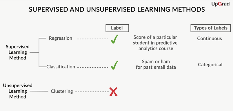
• Unsupervised learning wherein you try to identify patterns in data without being given a pre-determined set of labels.

• Common clustering algos
• K-Means
• Hierarchical

• Clustering considerations / Underlying philosophy
• Stability - class of members should not change if  clustering algo is run multiple times
• Inter-group heterogeneity & intra-group homogeneity is important. 
• Members of different segments/cluster should have distinctly different behaviour/traits
• Members of the same cluster/segment should have similar behaviour/trait.

• K-Means
• Customer Segmentation (typical criteria)
• Behavioral (based on customer actions)
• Attitudinal (based on customer intention e.g. brand-consciousness)
• Demographic (could be a good substitute/shortcut for Behavioral)
• Common practice of customer clustering is to use RFM as a triad of features on which to base clustering
• R - Recency (how recent have been a customer's purchases/interactions)
• F - Frequency (frequency of buying)
• M - Monetary value of purchases.
• Other segmentation practices
• RPI 
• Relationship  
• Persona (e.g gift-giver based on the fact that a person orders and mostly ships to other addresses)
• Intention (can be discerned based on browsing pattern)
• CDJ ( Consumer Decision Journey)
• Use a "Funnel" structure
• Hierarchical
• No need to pre-determine number of clusters
• Start with each point being a cluster and then iterate through to form one big cluster
• (Needs more processing power since it is more time-consuming)
• In the process create a dendrogram of the points at each step of cluster
• Clusters meeting at a higher point are more dissimilar
• Determine number of clusters by drawing a horizontal cut-off point across the dendrogram. Number of intersection points gives the # of clusters
• Cut-off line is somewhat arbitrary. Can be done bottom-up, called, agglomerative or top-down, called divisive.
• Linkage is the distance between points of one cluster to another in the process of fusing and creating clusters
• Single-linkage (take min distance between inter-cluster points)
• Complete-linkage (take max distance b/w inter-cluster points)
• Average-linkage (take avg distance b/w inter-cluster points)
• Clustering Choice Considerations

Confusion Matrix

Confusion Matrix

Actual/Predicted	Negative	Positive
Negative	TN	FP
Positive	FN	TP

• Accuracy
• fraction of correctly identified positives & negatives
  = TP + TN / TP+TN+FP+FN
• Sensitivity/ Recall / Hit Rate / True Positive Rate (TPR) 
• # of actual Yeses correctly predicted / Total # of actual Yeses
  = TP / (TP+FN)
• Specificity / Selectivity / True Negative Rate (TNR) 
• # of actual No's correctly predicted / Total # of actual Nos
  = TN / (TN+FP)
• Precision / Positive Predictive Value
• Probability that a predicted Yes is actually a Yes.
  = TP / (TP+FP)
• Score=400+(20∗log(odds)log(2))

• More metrics.

Principal Component Analysis

Principal Component Analysis

Is a linal based technique to reduce dimensionality of features while capturing the maximum information from the features. In other words, say, you have 10 features/variables describing a dataset. PCA helps one reduce the 10 features to a fewer number while capturing the effect of the all the variables without dropping any variable. This is important because, in techniques, like linear regression, we would normally compromise by dropping variables which have high multicollinearity. The PCA essentially compacts high multicollinear variables into one component, thereby reducing all features into a smaller set of "principal components" that affect the outcome. A key tenet in this is capturing the variance amongst variables in decreasing order of magnitude. That means there is an order to the principal components, with the first component explaining the effect on the outcome to the greatest extent and so on.

Practical Considerations

1. PCA is good with linear relationships, since it reduces variables to components that are expressed as a linear combination of the original variables (and hence good to use this on techniques such as logistics regression. Even otherwise PCA can be used for more efficient computation). However, in situations where you need non-linear treatment, the t-SNE (t-distributed Stochastic Neighbourhood Embedding) is an alternative although it is computationally intensive/prohibitive. Use it only when data is reasonably small. 
2. PCA assumes orthogonality to capture variances. Data may not be always be like that. In such situations, ICA (Independent Components Analyis) is a better option though it is again computationally intensive.
3. PCA de-emphasizes variables with low variance. This may not work well in situations where low-variance is also important, such as, fraud cases where data is small to begin with.

Deep Learning/Neural Network Applications

• Today, by far, Neural Network models seem to be among the top algos - based on competition results.
• Such models run into millions of parameters (still a fraction of the billions of neurons in the human brain)
• The network itself doesn't have intelligence, it is only through training (with TONS of data) that intelligence is gained.

Applications

1. Image recognition
2. Image tagging & video analysis
3. Auto text generation
4. Annotations for text & video
5. Speech recognition
6. Grammar change recommendations
7. Text translation
8. Automating games
9. Search text & draw inferences (such as an assistant for a Doctor/Lawyer etc.)

Natural Language Processing

Natural Language Processing

• NLP Model
• Lexical Processing (Basic text/word extraction that are most relevant to the topic/text at hand)
• Syntactic Processing (Understanding the grammar)
• Semantic Processing (Understanding the meaning)

• PMI
• Pointwise Mutual Information (PMI) is a metric that is used as part of advanced tokenisation techniques for identifying words in a text that collectively could be referring to a single entity (or term) . 
• It helps identify words that usually go together, representing a term/entity as opposed to treating them as independent words. 
• e.g "Indian Institute of Technology" - While each of the words Indian, Institute & Technology have their own meaning or standing, together they represent a single entity/term.
• PMI is calculated as follows
• pmi (x; y) = log (P(x,y) / P(x)P(y))
  where x & y are the individual words which collectively refer to a single term/entity
• i.e., log of probability of the words x & y occurring together, divided by the product of probabilities of x & y appearing/occurring separately.
• Syntactic Processing (steps)
• Parsing: Understanding various parts of a sentence and how they interplay with each other i.e. identifying verbs, nouns, subjects, objects etc.
• Parts of Speech (POS) tagging aka Shallow Parsing
• Constituency (or Paradigmatic) parsing
• Dependencies parsing
• Dependency grammar (as opposed to Constituency Parsing) can be traced back to Panini's grammar rules.
• Topic modelling
• This pertains to determining the topic of a given document, also called aboutness i.e., what is the document or a particular chunk of text about. 
• aboutness is not binary but is more of a degree of proximity. e.g. sugar can be about health, sugar industry, diabetes to varying degrees. 
• Topic modelling/extraction approaches
• PLSA - Probabilistic Latent Semantic Analysis
• LDA - Latent Dirichlet Allocation
• ESA - Explicit Semantic Analysis
• 
  
• NLP Resources
• dependency visualizer
• universal dependencies specs.
• stanford parser (dependency parser)
• converting list of tags into a tree
• dealing with incorrect POS tagging
• recursive descent parser
• 
  

Tree Models

All notes below are from Upgrad Course material

Pro's

• Decision trees model are most popular way of addressing classification problems
• Ease of interpretation:
  The decision trees are easy to interpret. Almost always, you can identify the various factors that lead to the decision. In fact, trees are often underestimated for their ability to relate the predictor variables to the predictions. As a rule of thumb, if interpretability by laymen is what you're looking for in a model, decision trees should be at the top of your list.
• Other models such as SVMs, logistics regression have a certain assumption of the data for them work effectively
• They need strictly numeric data
• Categorical data cannot be handled in a natural way
• Don't have the above limitation in terms of needing only numeric data.
• Don't need normalization of data.
• Decision trees often give us an idea of the relative importance of the explanatory attributes that are used for prediction.

Con's

• Decision trees tend to overfit the data. If allowed to grow with no check on its complexity, a tree will keep splitting till it has correctly classified (or rather, mugged up) all the data points in the training set.
• Decision trees tend to be very unstable, which is an implication of overfitting. A few changes in the data can change a tree considerably.

Dealing with Overfitting

There are two ways to control overfitting in trees:

• Truncation - Stop the tree while it is still growing so that it may not end up with leaves containing very few data points.
• Pruning - Let the tree grow to any complexity. Then, cut the branches of the tree in a bottom-up fashion, starting from the leaves. It is more common to use pruning strategies to avoid overfitting in practical implementations.

Truncation

Though there are various ways to truncate or prune trees, the DecisionTreeClassifier function in sklearn provides the following hyperparameters which you can control:

• criterion (Gini/IG or entropy): It defines the function to measure the quality of a split. Sklearn supports “gini” criteria for Gini Index & “entropy” for Information Gain. By default, it takes the value “gini”.
• max_features: It defines the no. of features to consider when looking for the best split. We can input integer, float, string & None value.
1. If an integer is inputted then it considers that value as max features at each split.
2. If float value is taken then it shows the percentage of features at each split.
3. If “auto” or “sqrt” is taken then max_features=sqrt(n_features).
4. If “log2” is taken then max_features= log2(n_features).
5. If None, then max_features=n_features. By default, it takes “None” value.
• max_depth: The max_depth parameter denotes maximum depth of the tree. It can take any integer value or None. If None, then nodes are expanded until all leaves are pure or until all leaves contain less than min_samples_split samples. By default, it takes “None” value.
• min_samples_split: This tells above the minimum no. of samples required to split an internal node. If an integer value is taken then consider min_samples_split as the minimum no. If float, then it shows percentage. By default, it takes “2” value.
• min_samples_leaf: The minimum number of samples required to be at a leaf node. If an integer value is taken then consider - -min_samples_leaf as the minimum no. If float, then it shows percentage. By default, it takes “1” value.

Neural Network Notational Symbols

Neural Network Notational Symbols

x  - input vector
h - hidden layer output vector
y - ground truth vector
p - predicted output probability vector

c - # of output classes
n - # of neurons (in a layer)

l - layer supersript

i - index subscript

s - index for a current layer neuron

t - index for the previous layer neuron

W - weight matrix (of a layer)

b - bias vector
σ - sigmoid (activation) function (applied on a layer). More generally, activation function need not be a sigmoid function.

z - cumulative weighted input going into a layer, on which the activation function is applied.

Backpropagation "Intuition"

For a 4-layer network
i.e., Input + 2 Hidden Layers + Output layer i.e., layers 0, 1, 2, 3.

1. dz^[3] i.e., differential of loss function w.r.t. to  z for layer 3 (output) =  (p - y) i.e., delta of predicted output and actual output (ground truth).
2. dW^[3] i.e., differential of loss function w.r.t to weights (w) for layer 3 (output) = dz^[3] . (h^[2])^T i.e., differential of loss function w.r.t. to z for layer 3 affected by (activated) output of layer 2.
   ----
3. dh^[2] i.e, differential of loss function w.r.t (activated) output for layer-2  = (W^[3])^T .  dz^[3]  i.e., weights going into layer-3 affected (multiplied) by differential of loss function w.r.t. to z for layer 3.
4. dz^[2]  i.e., differential of loss function w.r.t to z for layer-2 =   dh^[2] ⓧ  σ'(z^[2])  i.e., differential of loss function w.r.t to layer-2 output multiplied element-wise with differential of layer-2 (activated) output w.r.t to z for layer-2.
5. dW^[2] i.e., differential of loss function w.r.t to weights for layer 2  = dz^[2] . (h^[1])^T i.e., (activated) output of layer 1 affected (multiplied) by differential of loss function w.r.t z for layer-2.
   ----
6. dh^[1] i.e, differential of loss function w.r.t (activated) output for layer-1 = (W^[2])^T .  dz^[2]  i.e., weights for layer-2 affected (multiplied) by differential of loss function w.r.t. to z for layer 2.
7. dz^[1]  i.e., differential of loss function w.r.t to z for layer-1 =   dh^[1] ⓧ  σ'(z^[1])  i.e., differential of loss function w.r.t to layer-1 output multiplied element-wise with differential of layer-1 (activated) output w.r.t to z for layer-1.
8. dW^[1] i.e., differential of loss function w.r.t to weights for layer-1  = dz^[1] . (x)^T i.e., input layer  affected (multiplied) by differential of loss function w.r.t z for layer-1.

Backpropagation Algo (batch-based)

Firstly, note that the loss $L$ is computed over a batch. In a way, the batch acts as a proxy for the whole dataset. Hence, for a batch size of $m$, the average loss is:

$\frac{1}{m}{\sum }_{xϵB}L\left(N\right(x),y)$

This is the average loss over the $m$ data points of the batch. $N\left(x\right)$ is the network output (the vector $p$). Let's denote a batch of input data points by the matrix $B$. The backpropagation algorithm for a batch is:

1. $H^0=B$
2. for $l$ in $[1,2,.......,L]:$
   1. $H^l=\sigma (W^l.H^{l-1}+b^l)$
3. $P$ = $normalize(exp$($W^o.H^L+b^o$$\left)\right)$
4. $L=$$-\frac{1}{m}{Y}^T.log\left(P\right)$
5. $D{Z}^{L+1}$ =   $P-Y$
6.  $D{W}^{L+1}$ =  $D{Z}^{L+1}$.${\left(H^L\right)}^T$
7. for $l$ in $[L,L-1,........1]:$
   1.  $d{H}^l$ = $(W^{l+1}{)}^T.$$D{Z}^{l+1}$
   2. $D{Z}^l$ = $d{H}^l$$\otimes$${\sigma }^{\prime }\left(Z^l\right)$
   3.  $D{W}^l$ = $D{Z}^l.(H^{l-1}{)}^T$
   4.  $D{b}^l$  = $D{Z}^l$

Note that earlier $d{z}^l$represented a vector while $D{Z}^l$ now represents the matrix consisting of the $d{z}^l$vectors of all the data points in $B$ (each $d{z}^l$being a column of $D{Z}^l$). Similarly, $d{H}^l$, $Y$, $P$ and $H^l$ are all matrices of the corresponding individual vectors stacked side by side.