CNN: Working With Images: Summary Steps

1. Data Preparation: 
1. Make sure all images are of the same resolution.
2. Organize images into folders based on the class being predicted i.e, a folder for each class.
   
2. Data Pre-processing: Morphological Operations
1. Thresholding on the image - convert it from a grey image to a binary image.
2. Look at Erosion, Dilation, Opening, Closing.
   
3. Data Pre-processing: Normalisation
1. Divide by 255 (or) 
2. Divide by max-min (or)
3. Divide based on percentile (to account for outliers)
   
4. Data Pre-Processing: Augmentation
1. Two types of transformations for augmentation - linear and affine.
2. Different ways to augment - translation, rotation, scaling, etc.
3. Adds variability to add to train the model better.
   
5. Model Building
1. Run ablation experiments
2. Overfit on a smaller version of the training set
3. Hyperparameter tuning
4. Model training and evaluation

Custom Data Generator Code

• To start with, we have the training data stored in n directories (if there are n classes). For a given batch size, we want to generate batches of data points and feed them to the model.
• The first for loop 'globs' through each of the classes (directories). For each class, it stores the path of each image in the list paths. In training mode, it subsets paths to contain the first 80% images; in validation mode it subsets the last 20%. In the special case of an ablation experiment, it simply subsets the first ablation images of each class.
• We store the paths of all the images (of all classes) in a combined list self.list_IDs. The dictionary self.labels contains the labels (as key:value pairs of path: class_number (0/1)).
• After the loop, we call the method on_epoch_end(), which creates an array self.indexes of length self.list_IDs and shuffles them (to shuffle all the data points at the end of each epoch).
• The _getitem_ method uses the (shuffled) array self.indexes to select a batch_size number of entries (paths) from the path list self.list_IDs.
• Finally, the method __data_generation returns the batch of images as the pair X, y where X is of shape (batch_size, height, width, channels) and y is of shape (batch size, ). Note that __data_generation also does some preprocessing - it normalises the images (divides by 255) and crops the center 100 x 100 portion of the image. Thus, each image has the shape (100, 100, num_channels). If any dimension (height or width) of an image less than 100 pixels, that image is deleted.

import numpy as np
import keras

class DataGenerator(keras.utils.Sequence):
    'Generates data for Keras'
    
    def __init__(self, mode='train', ablation=None, flowers_cls=['daisy', 'rose'], 
                 batch_size=32, dim=(100, 100), n_channels=3, shuffle=True):
        """
        Initialise the data generator
        """
        self.dim = dim
        self.batch_size = batch_size
        self.labels = {}
        self.list_IDs = []
        
        # glob through directory of each class 
        for i, cls in enumerate(flowers_cls):
            paths = glob.glob(os.path.join(DATASET_PATH, cls, '*'))
            brk_point = int(len(paths)*0.8)
            if mode == 'train':
                paths = paths[:brk_point]
            else:
                paths = paths[brk_point:]
            if ablation is not None:
                paths = paths[:ablation]
            self.list_IDs += paths
            self.labels.update({p:i for p in paths})
            
        self.n_channels = n_channels
        self.n_classes = len(flowers_cls)
        self.shuffle = shuffle
        self.on_epoch_end()

    def __len__(self):
        'Denotes the number of batches per epoch'
        return int(np.floor(len(self.list_IDs) / self.batch_size))

    def __getitem__(self, index):
        'Generate one batch of data'
        # Generate indexes of the batch
        indexes = self.indexes[index*self.batch_size:(index+1)*self.batch_size]

        # Find list of IDs
        list_IDs_temp = [self.list_IDs[k] for k in indexes]

        # Generate data
        X, y = self.__data_generation(list_IDs_temp)

        return X, y

    def on_epoch_end(self):
        'Updates indexes after each epoch'
        self.indexes = np.arange(len(self.list_IDs))
        if self.shuffle == True:
            np.random.shuffle(self.indexes)

    def __data_generation(self, list_IDs_temp):
        'Generates data containing batch_size samples' # X : (n_samples, *dim, n_channels)
        # Initialization
        X = np.empty((self.batch_size, *self.dim, self.n_channels))
        y = np.empty((self.batch_size), dtype=int)
        
        delete_rows = []

        # Generate data
        for i, ID in enumerate(list_IDs_temp):
            # Store sample
            img = io.imread(ID)
            img = img/255
            if img.shape[0] > 100 and img.shape[1] > 100:
                h, w, _ = img.shape
                img = img[int(h/2)-50:int(h/2)+50, int(w/2)-50:int(w/2)+50, : ]
            else:
                delete_rows.append(i)
                continue
            
            X[i,] = img
          
            # Store class
            y[i] = self.labels[ID]
        
        X = np.delete(X, delete_rows, axis=0)
        y = np.delete(y, delete_rows, axis=0)
        return X, keras.utils.to_categorical(y, num_classes=self.n_classes)

CNN: Working with Images

Pre-Processing

Morphological Transformations

• Images come in different shapes and sizes. They also come from different sources. For example, some images are what we call “natural images”, which means they are taken in colour, in the real world. For example:
      A picture of a flower is a natural image.
      An X-ray image is not a natural image. 
• Natural images also have a specific statistical meaning ( Read this StackOverflow answer that describes this definition in some detail.
• Image Processing Technique: The term morphological transformation refers to any modification involving the shape and form of the images. These are very often used in image analysis tasks. Although they are used with all types of images, they are especially powerful for images that are not natural (come from a source other than a picture of the real world).
• RGB is the most popular encoding format, and most "natural images" we encounter are in RGB.
• Also, among the first step of data pre-processing is to make the images of the same size.
• Morphological transformations are applied using the basic structuring element called 'disk'.  A disk is defined with the code:
  selem = selem.disk(<n>)
• Thresholding: One of the simpler operations where we take all the pixels whose intensities are above a certain threshold, and convert them to ones; the pixels having value less than the threshold are converted to zero. This results in a binary image.
• Erosion, Dilation, Opening & Closing
• Erosion shrinks bright regions and enlarges dark regions. Dilation on the other hand is exact opposite side - it shrinks dark regions and enlarges the bright regions.
• Opening is erosion followed by dilation. Opening can remove small bright spots (i.e. “salt”) and connect small dark cracks. This tends to “open” up (dark) gaps between (bright) features.
• Closing is dilation followed by erosion. Closing can remove small dark spots (i.e. “pepper”) and connect small bright cracks. This tends to “close” up (dark) gaps between (bright) features.
• All these can be done using the skimage.morphology module. The basic idea is to have a circular disk of a certain size (3 below) move around the image and apply these transformations using it.

Normalisation

• Normalisation makes the training process much smoother. 
• Some Formulae for normalisations
• image / 255 
• (image - np.min(image))  /  (np.max(image) - np.min(image))
• (image - np.percentile(image,5)) / (np.percentile(image,95 - np.percentile(image,5)) Use this when you have outliers

Augmentation

• Reasons for Augmentation
• Small training dataset. No-brainer in this case since you don't have enough data to train the algo.
• Preventing overfitting. To prevent conv nets to learn/memorize images based on very specific patterns and location attributes on objects in an image. Hence distort images fairly to account fo tilting, angle etc.
• Pooling increases the invariance. If a picture of a dog is in the top left corner of an image, with pooling, you would be able to recognize if the dog is in little bit left/right/up/down around the top left corner. But with training data consisting of data augmentation like flipping, rotation, cropping, translation, illumination, scaling, adding noise etc., the model learns all these variations. This significantly boosts the accuracy of the model. So, even if the dog is there at any corner of the image, the model will be able to recognize it with high accuracy. 
• Types of Augmention
• Linear: Scale/Multiply image with a matrix
• Rotations, Flipping (horizontal & vertical) etc.
• Not all flipping operations are applicable always.
  E,g,. for a an x-ray, you want to be careful which flip operation you are using. OTOH, picture of a flower should be OK to be flipped any which way.
• Affine: More complex -> Translation + Linear 

Building the Network (ResNet)

Data Generator

• When dealing with large volume on input data (i.e., images), due to memory constraints, the technique of data generator is used
• Load only one set of images at a time (say, 5, 10 or 15). 
• Keep track of the last one processed in a set so as to be able to load the next set appropriately and so on.
• Keras comes with a DataGenerator class. However one can use a custom data generator class to be able to modify it according to the problem at hand (customizability).
  Custom Data Generator class (an example)

Ablation

Before training the net on the entire dataset, you should always try to first run some experiments to check whether the net is fitting on a small dataset or not.

Checking that the network is 'working'

• The first part of building a network is to get it to run on your dataset. 
• Try fitting the net on only a few images and just one epoch. 
• Tune hyperparameters.

Overfitting on the Training Data

• A good test of any model is to check whether it can overfit on the training data (i.e. the training loss consistently reduces along epochs). 
• This technique is especially useful in deep learning because most deep learning models are trained on large datasets, and if they are unable to overfit a small version, then they are unlikely to learn from the larger version.
• During training, sometimes you may get NaN as a loss instead of some finite number. This denotes that the output value predicted by the model is very high, which results in high loss value. 
• This causes exploding gradient problem. 
• The problem could be a high learning rate and to overcome, you can use SGD Optimiser. Although the adaptive methods (Adam, RMSProp etc.) have better training performance, they can generalize worse than SGD. 
• Furthermore, you can also play with some of the initialisation techniques like Xavier initialisation, He initialisation etc. 
• As a last resort, change the architecture of the network if the problem does not get solved. 
• This article lists some common ways in which you can prevent your ML model from overfitting.
• This paper compares various optimisers. 

Hyperparameter Tuning

• The basic idea is to track the validation loss with increasing epochs for various values of a hyperparameter (e.g. Learning Rate, Augmentation technique etc.)

Keras Callback

• Callbacks are basically actions that you want to perform at specific instances of training. For example, we want to perform the action of storing the loss at the end of every epoch (the instance here is the end of an epoch).
• Formally, a callback is simply a function (if you want to perform a single action), or a list of functions (if you want to perform multiple actions), which are to be executed at specific events (end of an epoch, start of every batch, when the accuracy plateaus out, etc.). Keras provides some very useful callback functionalities through the class keras.callbacks.Callback.
• Keras has many builtin callbacks (listed here). The generic way to create a custom callback in keras is:
  # generic way to create custom callbackclass LossHistory(keras.callbacks.Callback):        def on_train_begin(self, logs={}):               self.losses = []

        def on_batch_end(self, batch, logs={}):                   
            self.losses.append(logs.get('loss'))

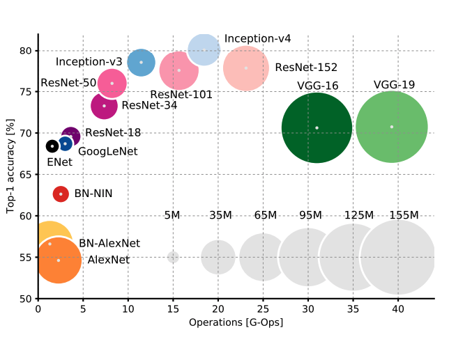
CNN Architectures: Comparative Study

Source:

An Analysis of Deep Neural Network Models for Practical Applications

Comparison dimensions

1. Number of model parameters
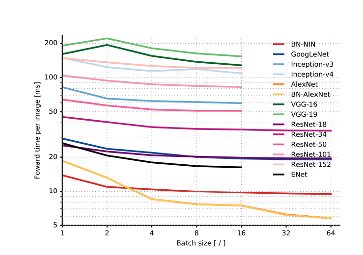
2. Time taken for inference (essentially feed forward)
3. Number of operations carried to do the inference 
4. Power consumption
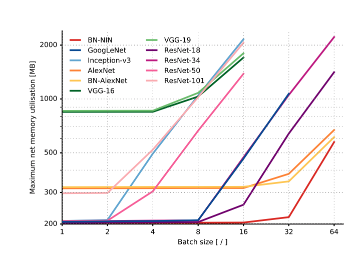
5. Relationship with Batch size

Practical Application Considerations

• Architectures in a particular cluster, such as GoogleNet, ResNet-18 and ENet, are very attractive since they have small footprints (both memory and time) as well as pretty good accuracies. Because of low-memory footprints, they can be used on mobile devices, and because the number of operations is small, they can also be used in real time inference.
• In some ResNet variants (ResNet-34,50,101,152) and Inception models (Inception-v3,v4), there is a trade-off between model accuracy and efficiency, i.e. the inference time and memory requirement. 
• Most, if not all, models seem to have marginal improvement in time for inference as batch size is increased (except AlexNet)
• Power consumption for most models is around the same.
• Beyond a certain batch size, memory increases (shoots up) linearly with batch size. Until then, memory req is quite low. Thus, it might not be a bad idea to use a large batch size if you need to. 
• Up to a certain batch size, most architectures use a constant memory, after which the consumption increases linearly with the batch size.
• Accuracy and inference time are in a hyperbolic relationship: a little increment in accuracy costs a lot of computational time
• Power consumption is independent of batch size and architecture. 
• The number of operations in a network model can effectively estimate inference time.
• ENet is the best architecture in terms of parameters space utilisation

Deep Learning Jots

Source: https://papers.nips.cc/paper/4824-imagenet-classification-with-deep-convolutional-neural-networks.pdf

• Despite the attractive qualities of CNNs, and despite the relative efficiency of their local architecture, they have still been prohibitively expensive to apply in large scale to high-resolution images. Luckily, current GPUs, paired with a highly-optimized implementation of 2D convolution, are powerful enough to facilitate the training of interestingly-large CNNs, and recent datasets such as ImageNet contain enough labeled examples to train such models without severe overfitting.
• A four-layer convolutional neural network with ReLUs reaches a 25% training error rate on CIFAR-10 six times faster than an equivalent network with tanh neurons (dashed line). 
• Networks with ReLUs consistently learn several times faster than equivalents with saturating neurons.
• 1.2 million training examples are enough to train networks which are too big to fit on one GPU (A single GTX 580 GPU has only 3GB of memory).
• The easiest and most common method to reduce overfitting on image data is to artificially enlarge the dataset using label-preserving transformations.
• Top-1 Error means the proportion of incorrectly classified images;
• Top-5 Error means the proportion of images such that the ground-truth category is outside the top-5 predicted categories

Convolutional Neural Networks (CNNs)

• Inspired by the animal/human visual system
• Primarily created to handle visual recognition but has since found wider applications.

Key Features of a CNN Architecture

• Each unit, or neuron, is dedicated to its own receptive field. Thus, every unit is meant to ignore everything other than what is found in its own receptive field.
• The receptive field of each neuron is almost identical in shape and size.
• The subsequent layers compute the statistical aggregate of the previous layers of units. This is analogous to the 'pooling layer' in a typical CNN.
• Inference or the perception of the image happens at various levels of abstraction. The first layer pulls out raw features, subsequent layers pull out higher-level features based on the previous features and so on. Finally, the network gets an overall perception of an image in the last layer.

Components of a CNN

VGGNet is a pure implementation of a CNN.

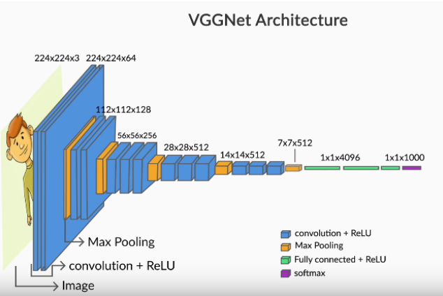
• Convolution
• Pooling Layers
• Feature Maps

Convolution

• Process of applying a filter on an image to get a specific, specialised perspective of the image. 
• A filter is a somewhat arbitrary matrix of numbers, which is smaller than the image matrix
• The filter is applied or scanned on the entire image.
• The convolution process essentially does an element-wise multiplication between the image pixel numbers and the filter numbers and sums them up. 
• Hence a 6x6 image when convolved with a 3x3 filter will yield a 4x4 matrix since the filter can be placed in 4 different horizontal & vertical positions each on the original image.

Padding Calculation to maintain post-convolution input size

The output size is $\frac{n+2p-k}{s}+1$. With p=1, k=3, s=1, the output will always be (n, n).  

Model Selection

Key Points on Model Selection

• Central question for any ML model is
  How to extrapolate learnings from a finite amount of data to explain or predict all possible inputs of the same kind
• Domain knowledge is a very important factor in making decisions on ML Models for a given problem.
• Usefulness of a model is determined by how it performs unseen data 
• Occam's razor is perhaps the most important thumb rule in machine learning, and incredibly 'simple' at the same time. When in dilemma, choose the simpler model.
• Logistic regression is simple to run, with no hyperparameters to tune. It can be used as a benchmark to compare the performance of other models.
• Support vector machines can take quite a bit of time to run because of their resource-intensive nature. It also takes multiple runs to choose the best kernel for a particular problem.
• A decision tree generally does not perform well on a dataset with a lot of continuous variables. Since the tree is performing well on the dataset, it is highly unlikely that the data has only continuous attributes.
• If the difference between training and validation accuracy is significant, then you can conclude that the tree has overfitted the data.
• A logistic regression model can also work with nonlinear separable datasets, but the performance will not be at par with other machine learning models such as decision trees, SVMs etc.

Comparison of Models

Logistic Regression (LR), Decision Trees & SVMs

Logistic Regression

Pro’s	Con’s
Logistic Regression
t is convenient for generating probability scores. 2.     Efficient implementation is available across different tools. 3.     The issue of multicollinearity can be countered with regularisation. 4.     It has widespread industry use.	It does not perform well when the features space is too large. It does not perform well when there are a lot of categorical variables in the data. The nonlinear features have to be transformed to linear features in order to efficiently use them for a logistic model. It relies on entire data i.e. if there is even a small change in the data, the logistic model can change significantly.
Decision Trees
Intuitive decision rules make it easy to interpret. Trees handle nonlinear features well. The variable interaction is taken into account.	Trees are highly biased towards the training set and overfit it more often than not. There is no meaningful probability score as the output
SVMs
SVMs can handle large feature space. These can handle nonlinear feature interaction. They do not rely on the entire dimensionality of the data for the transformation.	SVMs are not efficient in terms of computational cost when the number of observations is large. It is tricky and time-consuming to find the appropriate kernel for a given data.

CART and CHAID Trees

• Use CART for forecasting/prediction v/s CHAID which is better suited for driver analysis, i.e, understanding the key variables/features driving the behavior of the data/target.
  e,g., Suppose you are working with the Indian cricket team, and you want to predict whether the team will win a particular tournament or not. In this case, CART would be more preferable because it is more suitable for prediction tasks. Whereas, if you want to look at the factors that are going to influence the win/loss of the team, then a CHAID tree would be more preferable.

Decision Trees v/s Random Forest 

• Trees have a tendency to overfit the training data whereas with Random Forest trees, it is hard to overfit the data it uses bagging along with sampling the features randomly at each node split. This prevents them from overfitting the data, unlike decision trees.
• There is no need to prune trees in a random forest because even if some trees overfit the training set, it will not matter when the results of all the trees are aggregated.
• In a decision tree, while building a decision tree, at every node we introduce a condition (example: age>=20) on a feature which in turn creates a "linear" boundary perpendicular to that feature (age) to split the dataset into two. The number of such linear boundaries increases if the data is not linearly separable and more than one node have to be created for each features. Hence creating large number of  linear boundaries for highly non-linear data may not be efficient enough to classify the data points correctly.
• With any decision tree (even if using Random Forests), it is not possible to predict beyond the range of the response variable in the training data in a regression problem. Suppose you want to predict house prices using a decision tree and the range of the the house price (response variable) is $5000 to $35000. While predicting, the output of the decision tree will always be within that range. If unseen data has values outside this range, the model can be inaccurate.
• With a RF, the OOB error can be calculated from the training data itself which gives a good estimate of the model performance on unseen data.
• A random forest is not affected by outliers as much because of the aggregation strategy.

Limitations of Random Forest

• Owing to their origin to decision trees, random forests have the same problem of not predicting beyond the range of the response variable in the training set.
• Extreme values are often not predicted because of the aggregation strategy.
  To illustrate this, let’s take the house prices example, Where the response variable is the price of a house. 
• Suppose the range of the price variable is between $5000 and $35000. 
• You train the random forest and then make predictions. While making predictions for an expensive house, there will be some trees in the forest which predict the price of the house as $35000, but there will be other trees in the same forest with values close to $35000 but not exactly $35000. 
• In the end, when the final price is decided by aggregating using the mean of all the predictions of the trees of the forest, the predicted value will be close to the extreme value of $35000 but not exactly $35000. 
• Unless all the trees of the forest predict the house price to be $35000, this extreme value will not be predicted.

Directed v/s Undirected (Probability) Graphs

• If the relationship (between variables) that we are trying to model needs to be asymmetric (i.e. one variable influences the other but not the other way), then go for Directed model. 
• e.g. disease & symptom, drug & cure.
• If symmetric, then use Undirected model.
• e.g. pixels in an image.

How to build different models and choose the best

• Start with logistic regression. Using a logistic regression model serves two purposes: 
• It acts as a baseline (benchmark) model. 
• It gives you an idea about the important variables.
• Then, go for decision trees and compare their performance with the logistic regression model. If there is no significant improvement in their performance, then just use the important variables drawn from the logistic regression model.
• While building a decision tree, you should choose the appropriate method: CART for predicting and CHAID for driver analysis. 
• Finally, if you still do not meet the performance requirements, and you have sufficient time & resources on hand, then go ahead and build more complex models like random forests & support vector machines. 
• In general, starting from a basic model helps in two ways: 
1. If the model performs as per requirement, there is no need to go to complex models. This saves time and resources. 
2. If it does not perform well, it can be used to benchmark the performance of other models.

Restricted Boltzman Machine

A restricted Boltzmann Machine is an "Energy Based" generative stochastic model. Initially invented by Paul Smolensky in 1986 and were called "Harmonium". After the evolution of training algorithms in the mid 2000's by Geoffrey Hinton, the boltzman machine became more prominent. It gained big popularity in recent years in the context of the Netflix Prize where RBMs achieved state of the art performance in collaborative filtering and have beaten most of the competition.

RBM's are useful for dimensionality reduction, classification, regression, collaborative filtering, feature learning and topic modeling.